Abstract
We implement a quantum algorithm for solving the Simple Harmonic
Oscillator (SHO) using the
Linear Combination of Unitaries (LCU)
framework from Xin et al. (2020). By approximating the matrix
exponential \( e^{At} \) via a Taylor expansion and encoding the
coefficients as a quantum superposition, we recover position and
velocity trajectories on a 4-qubit circuit that closely track the
classical solution, with
energy conservation
confirmed throughout.
A systematic parameter study identifies
\(k = 5\) Taylor terms, bound of
\(0.01\), and
\(n_{\text{shots}} = 8192\). as the
optimal operating point, balancing accuracy against circuit depth.
Our SHO serves as a minimal working example of an algorithm directly
applicable to larger first-order linear systems, including protein
dynamics and heat conduction.
Introduction
"Nature isn't classical, dammit, and if you want to make a
simulation of nature, you'd better make it quantum mechanical.", Richard Feynman, 1981
What do bungee jumping and playing guitar have in common? If fear was
the first answer that came to mind, we highly recommend looking for a
new guitar instructor.
Jokes aside, from a physics perspective both are real-world
applications of the
Simple Harmonic Oscillator, which we
abbreviate here as SHO. The SHO is one of the most universal models in
physics: it describes a system where a restoring force pulls an object
back toward equilibrium. The mathematical description of the motion of
a bungee jumper bouncing in the air is then identical to how we would
model a guitar string being plucked.
Although this mathematical formulation has been studied extensively,
in this notebook we explore a SHO system through a different lens and
learn to implement a
quantum algorithm
to solve this classical problem. Let's bungee jump right into it!
The Simple Harmonic Oscillator
A Simple Harmonic Oscillator is mathematically described by a
second-order linear differential equation:
$$\frac{d^2y}{dt^2} + \omega^2 y = 0 \tag{1}$$
This equation describes how the oscillator accelerates over time. \(
\omega \) is called the
angular frequency
and determines how fast the system oscillates. For example, a stiff
cord with high \( \omega \) means a bungee jumper will bounce faster,
and a guitar player that plucks a short and tight string will produce
a higher pitch note.
The second-order LDE in (1) can be reduced to a first-order LDE by
changing variables, where \( v = \frac{dy}{dt} \):
$$\frac{dy}{dt} = v, \quad \frac{dv}{dt} = -\omega^2 y \tag{2}$$
We make this substitution because this specific first-order LDE
appears across a remarkably wide range of physical contexts, governing
systems from climate modelling to fluid dynamics to quantum chemistry.
It allows us to study and solve the SHO via a well-studied classical
equation and reduces our system to just two variables:
position and
velocity.
Having only two variables simplifies our equation, as it has an exact
analytical solution. Note that more complex systems requiring many
variables quickly become computationally intractable for classical
computers, making them natural candidates for quantum algorithms.
Classically, the solutions are:
$$y(t) = \cos(\omega t) + \sin(\omega t) \tag{3}$$
$$v(t) = -\omega\sin(\omega t) + \omega\cos(\omega t) \tag{4}$$
We will use these classical solutions to benchmark and validate our
quantum algorithm. If we can verify that the quantum algorithm works
with our SHO, we can extend it to systems anywhere this equation
appears, and it appears in many places.
Problem Statement
In this notebook, we aim to solve a Simple Harmonic Oscillator that
has the following properties and initial conditions:
$$\frac{d^2y}{dt^2} + \omega^2 y = 0, \quad y(0) = 1, \quad
\frac{dy}{dt}\bigg|_{t=0} = 1, \quad \omega = 1 \tag{5}$$
via the quantum algorithm proposed in the paper
"A Quantum Algorithm for Solving Linear Differential Equations:
Theory and Experiment"
by Tao Xin et al. (2020).
Quantum computers operate on vectors and matrices, so we rewrite (5)
in matrix form. With \(\omega = 1\):
$$\frac{d}{dt}\begin{pmatrix} y \\ v \end{pmatrix} = \begin{pmatrix} 0
& 1 \\ -1 & 0 \end{pmatrix} \begin{pmatrix} y \\ v \end{pmatrix},
\quad \mathbf{x}(0) = \begin{pmatrix} 1 \\ 1 \end{pmatrix} \tag{6}$$
where the matrix is:
$$A = \begin{pmatrix} 0 & 1 \\ -1 & 0 \end{pmatrix} \tag{7}$$
The solution to this LDE is:
$$\mathbf{x}(t) = e^{At}\mathbf{x}(0) \tag{8}$$
Since computing \(e^{At}\) exactly is hard, we approximate it using a
Taylor expansion:
$$e^{At} \approx \sum_{m=0}^{k} \frac{(At)^m}{m!} \tag{9}$$
Each term \(A^m \mathbf{x}(0)\) corresponds to applying the gate \(A\)
exactly \(m\) times to the initial state. Including more Taylor terms
increases the accuracy of the approximation, but also requires more
quantum gates to implement.
Solution Approximation
The Taylor coefficients are computed as:
$$C_m = \|\mathbf{x}(0)\| \cdot \frac{(\|A\| \cdot t)^m}{m!}, \quad m
= 0, 1, \ldots, k \tag{10}$$
which are then normalized to probabilities \(p_m = C_m / \sum_m C_m\).
Notice how the first few powers of \(A\) follow a cyclic pattern
(period 4):
$$A^0 = \begin{pmatrix} 1 & 0 \\ 0 & 1 \end{pmatrix}, \quad A^1 =
\begin{pmatrix} 0 & 1 \\ -1 & 0 \end{pmatrix}, \quad A^2 =
\begin{pmatrix} -1 & 0 \\ 0 & -1 \end{pmatrix}, \quad A^3 =
\begin{pmatrix} 0 & -1 \\ 1 & 0 \end{pmatrix} ... \tag{11}$$
Then the cycle repeats: \(A^4 = A^0\), \(A^5 = A^1\), and so on.
Let's calculate the Taylor coefficients at \(t = 0.5\),
\(\|\mathbf{x}(0)\| = \sqrt{2}\), \(\|A\| = 1 \tag{12}\), to
understand how much each term contributes to the approximation:
| \(m\) |
\(C_m\) |
\(p_m\) |
| 0 |
1.4142 |
0.6065 |
| 1 |
0.7071 |
0.3033 |
| 2 |
0.1768 |
0.0758 |
| 3 |
0.0295 |
0.0126 |
| 4 |
0.0037 |
0.0016 |
| 5 |
0.0004 |
0.0002 |
| 6 |
0.00003 |
~0 |
| 7 |
0.000002 |
~0 |
| 8 |
~0 |
~0 |
| 9 |
~0 |
~0 |
| 10 |
~0 |
~0 |
Notice how the coefficients decay rapidly due to the \(m!\) in the
denominator, and by \(m = 5\) they are already negligible. This is why
\(k = 5\) is sufficient for \(t \in [0, 1]\): the remaining terms
contribute less than 0.01% to the sum.
As first assumption, we can say
\(k = 5\) is a sufficient cutoff for
our Taylor expansion.
Unitarity
About Qubits
A qubit is the fundamental unit of
information in quantum computing. Unlike a classical bit which is
always 0 or 1, a qubit can exist in a
superposition of both states
simultaneously, as a weighted combination that only resolves to a
definite value upon measurement. This, combined with
entanglement, enables exponential
speedups for specific problem classes that are intractable for
classical computers.
Qubits are delicate physical systems (such as trapped ions or
superconducting circuits) that exist in fragile superposition states
and are extremely sensitive to environmental noise. Even tiny
disturbances can cause decoherence,
collapsing the quantum state and introducing errors. This makes them
notoriously difficult to build, control, and scale.
Quantum Gates and Unitarity
Quantum computers fundamentally rely on the implementation of
quantum gates. You can think of a
quantum gate as a matrix operation that transforms the state of one or
more qubits. An important characteristic of these matrices is that, to
be valid quantum operators, they need to be
unitary. Unitarity preserves the
total probability of the quantum states.
Mathematically, a matrix \(U\) is unitary if:
$$U^\dagger U = I \tag{12}$$
For our problem, the gates are the powers of \(A\). Let's verify that
\(A\) is unitary:
$$A^\dagger A = \begin{pmatrix} 0 & -1 \\ 1 & 0 \end{pmatrix}
\begin{pmatrix} 0 & 1 \\ -1 & 0 \end{pmatrix} = \begin{pmatrix} 1 & 0
\\ 0 & 1 \end{pmatrix} = I \checkmark \tag{13}$$
Since \(A\) is unitary, all its powers are too. We can verify this for
the first few powers:
$$A^0 = I = \begin{pmatrix} 1 & 0 \\ 0 & 1 \end{pmatrix}, \quad
(A^0)^\dagger A^0 = I \checkmark \tag{14}$$
$$A^1 = \begin{pmatrix} 0 & 1 \\ -1 & 0 \end{pmatrix}, \quad
(A^1)^\dagger A^1 = \begin{pmatrix} 0 & -1 \\ 1 & 0 \end{pmatrix}
\begin{pmatrix} 0 & 1 \\ -1 & 0 \end{pmatrix} = \begin{pmatrix} 1 & 0
\\ 0 & 1 \end{pmatrix} = I \checkmark \tag{15}$$
$$A^2 = \begin{pmatrix} -1 & 0 \\ 0 & -1 \end{pmatrix}, \quad
(A^2)^\dagger A^2 = \begin{pmatrix} -1 & 0 \\ 0 & -1 \end{pmatrix}
\begin{pmatrix} -1 & 0 \\ 0 & -1 \end{pmatrix} = \begin{pmatrix} 1 & 0
\\ 0 & 1 \end{pmatrix} = I \checkmark \tag{16}$$
$$A^3 = \begin{pmatrix} 0 & -1 \\ 1 & 0 \end{pmatrix}, \quad
(A^3)^\dagger A^3 = \begin{pmatrix} 0 & 1 \\ -1 & 0 \end{pmatrix}
\begin{pmatrix} 0 & -1 \\ 1 & 0 \end{pmatrix} = \begin{pmatrix} 1 & 0
\\ 0 & 1 \end{pmatrix} = I \checkmark \tag{17}$$
Therefore each \(A^m\) can be directly implemented as a quantum gate
without further decomposition. This places us in Case I of Tao Xin et
al., the simplest and most efficient case of the algorithm.
However, the Taylor expansion itself:
$$e^{At} \approx \sum_{m=0}^{k} \frac{(At)^m}{m!} = C_0 I + C_1 A +
C_2 A^2 + \cdots \tag{18}$$
is a weighted sum of unitaries, and a
sum of unitary matrices is generally
not unitary. We therefore cannot
implement it as a single quantum gate directly.
This is precisely why we resort to the
Linear Combination of Unitaries (LCU)
framework, a technique designed to implement exactly this kind of
weighted sum on a quantum computer, which we describe in the next
section.
Building the Circuit
We implement the
Linear Combination of Unitaries (LCU)
framework using Classiq, a quantum software platform that handles
circuit synthesis and optimization automatically, allowing us to
describe the algorithm at a high level without manually decomposing
every gate.
Given the delicate nature of qubits, a crucial initial step in a
quantum algorithm is
state preparation, where qubits are
initialized to a known, specific starting state before any computation
occurs. Think of it as clearing the memory of a computer and setting
all variables to zero, but in quantum terms, this is much more
complex.
Classiq easily interfaces the preparation of qubits. It uses an
ancilla or
controller register, which is like a
scratch pad that annotates which unitary operators in the linear
combination are to be applied, and a
work register as the system of qubits
that stores the final state.
In particular, the LCU framework is built around three components:
-
First, prepare loads the normalized
Taylor coefficients as a quantum superposition on the controller
register, so the quantum computer knows how much of each \(A^m\) to
apply. This is implemented via Classiq's
inplace_prepare_state, which takes the probabilities and a
bound parameter controlling the approximation error of the state
preparation. We set the bound to initially be
0.01, per Classiq default.
-
Then select applies the correct
power of \(A\) to the work register, controlled on the initial
state. Under the hood, the quantum computer applies each \(A^m\) as
a unitary gate, effectively implementing our Taylor series
approximation.
-
Finally, prepare† uncomputes the
controller register. Classiq handles this automatically via
within_apply.
The number of qubits in the state preparation is determined
dynamically by \(k\):
$$n_{\text{controller}} = \lceil \log_2(k+1) \rceil \tag{19}$$
Since we need to index \(k+1\) terms, the controller register grows in
discrete jumps; for example, \(k=1\) requires 1 controller qubit,
\(k=2,3\) require 2, and \(k=4\) jumps to 3, which directly impacts
circuit depth and width.
Here are the key steps in implementing the LCU for our oscillator:
def build_circuit(bound, probs_controller, k, A_powers):
    n_qubits_controller = math.ceil(math.log2(k + 1))

    @qfunc
    def prepare(controller: QNum) -> None:
        inplace_prepare_state(probs_controller, bound=bound, target=controller)

    @qfunc
    def select(controller: QNum, work: QArray) -> None:
        for m in range(k + 1):
            control(
                ctrl=controller == m,
                stmt_block=lambda m=m: unitary(elements=A_powers[m], target=work),
            )

    @qfunc
    def main(controller: Output[QNum], work: Output[QArray]) -> None:
        allocate(n_qubits_controller, controller)
        allocate(1, work)  # 1 qubit for 2D initial state, v and y

        # Prepare initial state |x(0)>
        inplace_prepare_state(probabilities=probs_x0, bound=bound, target=work)

        # LCU: PREPARE → SELECT → PREPARE†, where PREPARE† is automatically applied
        within_apply(
            within=lambda: prepare(controller),
            apply=lambda: select(controller, work),
        )

    return main
Post Selection and Measurement
After the LCU circuit runs, we measure both the work and controller
registers. The key step is
post-selection: we keep only the
shots where the controller register returns to \( |0\rangle \), which
are the successful LCU outcomes where the Taylor sum was correctly
applied.
After post-selection, the work register encodes the solution state:
$$|\mathbf{x}(t)\rangle \propto y(t)|0\rangle + v(t)|1\rangle
\tag{20}$$
So measuring \( |0\rangle \) corresponds to position \( y(t) \) and
measuring \( |1\rangle \) corresponds to velocity \( v(t) \). From the
measurement probabilities we recover:
$$y(t) = \text{sign}(y_{\text{cl}}) \cdot \sqrt{p_0} \cdot
\|\mathbf{x}(0)\| \tag{21}$$
$$v(t) = \text{sign}(v_{\text{cl}}) \cdot \sqrt{p_1} \cdot
\|\mathbf{x}(0)\| \tag{22}$$
Since quantum measurement yields
probabilities, not amplitudes, we
adjust the sign by comparing to the classical solution. This is a
standard limitation of quantum algorithms that encode information in
amplitudes rather than probabilities.
Finally, not all shots survive post-selection. The success rate:
$$r = \frac{\text{post-selected shots}}{\text{total shots}} \approx
\frac{1}{\mathcal{N}^2}, \quad \mathcal{N} = \sum_{m=0}^{k} C_m
\tag{23}$$
Decreases as \( t \) grows, since the Taylor sum \( \mathcal{N} \)
grows with \( t \).
Sources of Errors
Our quantum solution accumulates error from three distinct sources:
-
Taylor truncation error: since we
approximate \( e^{At} \) with a finite sum of \( k+1 \) terms, the
truncation error grows with \( t \) and shrinks with \( k \). This
is why accuracy declines at large \( t \) for small \( k \).
-
Shot noise: after post-selection,
the remaining shots are split between \( |0\rangle \) and \(
|1\rangle \) outcomes. Each probability estimate carries
statistical uncertainty that propagates through to the recovered
amplitudes \( y(t) \) and \( v(t) \). More post-selected shots
means lower shot noise.
-
Post-selection noise: not all
shots survive post-selection. The success rate decreases as \( t
\) grows, since the Taylor sum \( \mathcal{N} \) grows with \( t
\). This reduces the effective number of shots and amplifies shot
noise.
Results and Analysis
Now that we have set up our quantum circuit simulator, we are ready to
collect and analyse the data!
We start by ensuring the total energy of the system is preserved, and
we subsequently perform a parameter study.
For our initial measurements, we truncate our Taylor approximation to
the fifth term
k = 5, and we use the default Classiq
bound = 0.01 in the state preparation
step. We also use n_shots = 8192,
meaning that we repeat the measurement 8192 times and average over all
measurements.
Conservation of Energy
After we calculate \(y(t)\) and \(v(t)\), the energies follow
directly:
$$E_k = \frac{1}{2}v^2, \quad E_p = \frac{1}{2}\omega^2 y^2, \quad E =
E_k + E_p \tag{24}$$
For a perfect SHO, \(E\) is conserved and any deviation is a direct
measure of the algorithm's error.
We use standard error propagation:
$$\sigma_{E_k} = |v|\sigma_v, \quad \sigma_{E_p} = |y|\sigma_y, \quad
\sigma_E = \sqrt{\sigma_{E_k}^2 + \sigma_{E_p}^2} \tag{25}$$
We measure on \(t \in [0, 1]\) with 21 equally spaced time steps, and
observe:
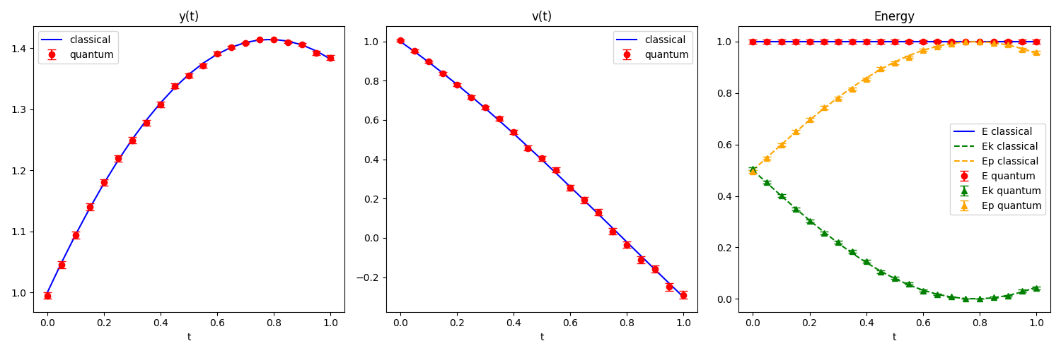
Observations
The quantum results closely track the classical solution for both
position and velocity. Total energy \( E(t) \) remains approximately
flat, confirming that the algorithm correctly follows energy
conservation!
Parameter Study: Bound
The bound parameter is
specific to Classiq's
inplace_prepare_state
function and controls the approximation error of the state preparation
circuit. It is not part of the original algorithm from Tao Xin et al.,
but rather a compilation parameter introduced by the Classiq platform.
We investigate its effect to ensure our choice of bound = 0.01 (the
Classiq default) does not compromise our results.
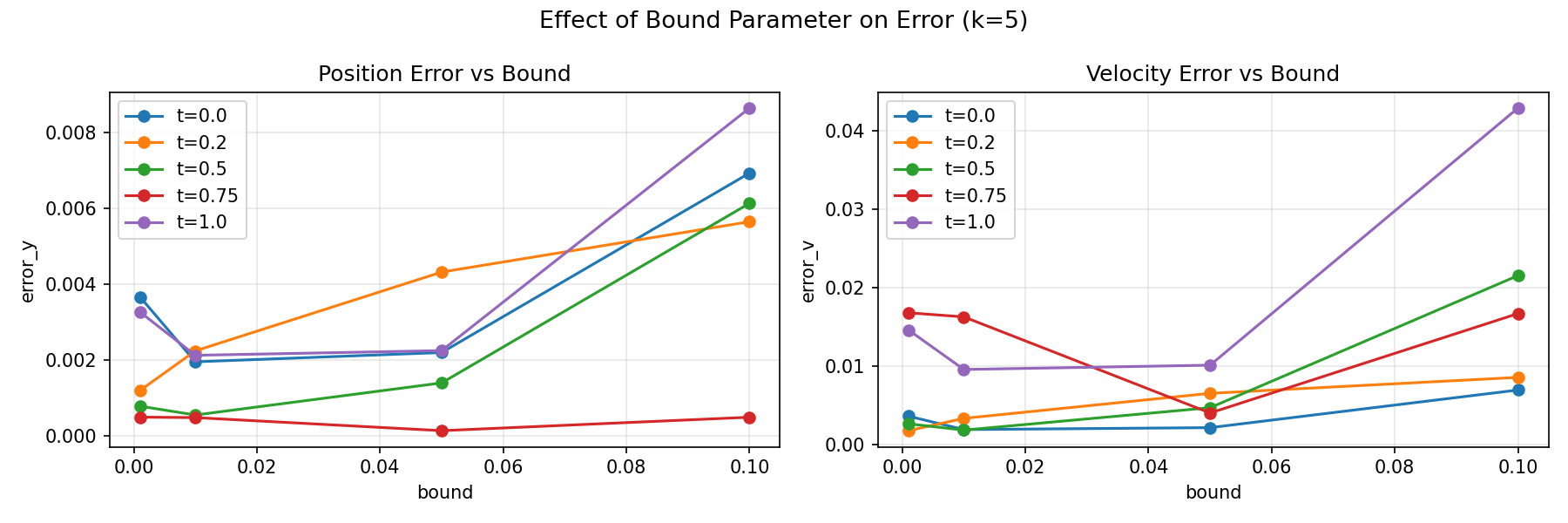
The position and velocity errors show no systematic dependence on
bound, as the lines fluctuate randomly rather than trending up or down
as bound increases. The magnitude of these fluctuations (\(\sim
0.001\!-\!0.01\)) is consistent with shot noise error.
Observations
This confirms that bound does not affect accuracy for this problem.
The Taylor coefficient distribution at \(k=5\) is sparse enough that
Classiq compiles essentially the same state preparation circuit
regardless of the bound parameter.
We therefore fix bound = 0.01 for all subsequent analysis.
Parameter Study: Taylor Approximation Cutoff
Having established that bound has no meaningful effect on our results,
we now investigate the effect of the Taylor truncation order \(k\).
Recall that \(k\) controls how many terms we include in the Taylor
expansion of \(e^{At}\):
$$e^{At} \approx \sum_{m=0}^{k} \frac{(At)^m}{m!} \tag{18}$$
We fix the bound to 0.01 and sweep \(k \in \{1, 2, 3, 4, 5, 6, 7,
8\}\) across five time points \(t \in \{0, 0.25, 0.5, 0.75, 1.0\}\).
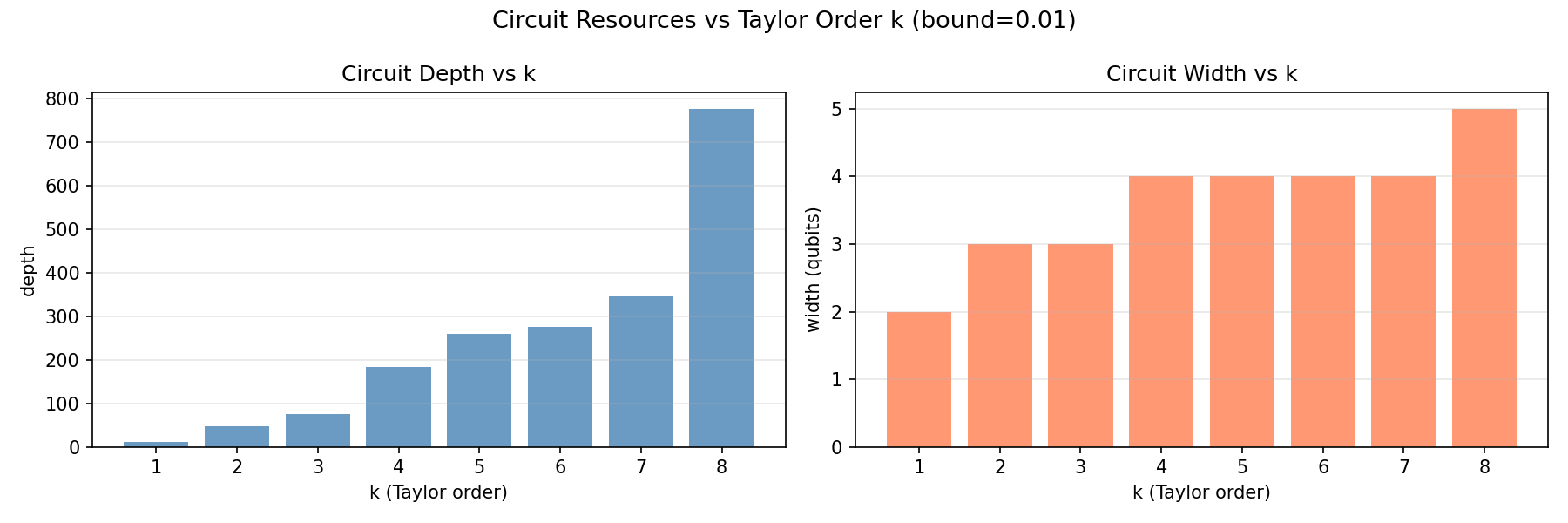
Circuit Resources
Width is the number of qubits
used, you can think of it as the memory of the circuit.
Depth is the number of
sequential gate layers, effectively the runtime.
⚠️ Note
Deeper circuits take longer to execute and accumulate more errors due
to decoherence.
Both width and depth grow with \(k\) in discrete jumps, explained by
the controller register size in (19):
$$n_{\text{controller}} = \lceil \log_2(k+1) \rceil \tag{19}$$
Width grows as \(\mathcal{O}(\log k)\) and depth as \(\mathcal{O}(k
\log k)\).
| \(k\) |
\(n_{\text{controller}}\) |
depth |
width |
| 1 |
1 |
~11 |
2 |
| 2 |
2 |
~50 |
3 |
| 3 |
2 |
~80 |
3 |
| 4–7 |
3 |
~180–350 |
4 |
| 8 |
4 |
~780 |
5 |
Accuracy
Accuracy improves with \(k\) as more Taylor terms better approximate
\(e^{At}\), but only until the truncation error falls below the shot
noise floor. Beyond that, adding more terms yields no measurable
improvement.
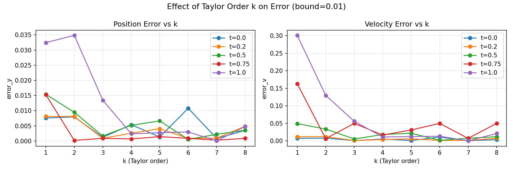
Interestingly, \(k=2\) shows higher error than \(k=1\) for \(t=1.0\),
likely due to the cyclic pattern of \(A^m\), since the even powers of
\(A\) are \(-I\), which can temporarily worsen the approximation
before higher-order terms correct it.
Observations
\(k=5\) is the optimal operating point, as it sits within the 4-qubit
regime, achieves good accuracy across \(t \in [0,1]\), and avoids the
expensive depth jump at \(k=8\).
Parameter Study: Number of Shots
We first compare the observed post-selection rate to the theoretical
prediction \(1/\mathcal{N}^2\) across time:
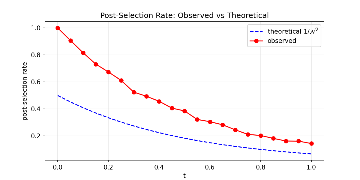
We observe that the post-selection rate is consistently higher than
the theoretical \(1/\mathcal{N}^2\) prediction. This is expected, as
the formula from Tao Xin et al. is a
lower bound. Both curves decrease with \(t\), confirming the theoretical trend.
Next, we fix k = 5 and bound = 0.01 and sweep \(n_{\text{shots}} \in
\{256, 1024, 4096, 8192\}\) across 21 time steps \(t \in [0, 1]\).
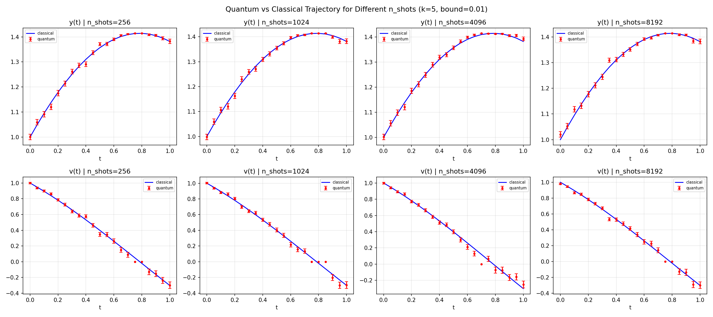
Observations
All four panels look almost identical, confirming that shot noise is
not the bottleneck at \(k=5\). Error bars shrink slightly from
\(n=256\) to \(n=8192\), but trajectory accuracy does not meaningfully
improve. The degradation of \(v(t)\) at large \(t\) persists across
all shot counts, confirming that
Taylor truncation is the dominant error source, not shot noise.
We therefore fix \( n_{\text{shots}} = 8192 \) as a safe default!
Optimal Operating Parameters
We verified that for a perfect SHO, the total energy is conserved at
all times. This is the bungee jumper's energy budget: as she falls,
kinetic energy increases while potential energy decreases, and the
total stays constant. Any deviation in \(E(t)\) from our quantum
algorithm is a direct, physical measure of algorithmic error. If our
quantum solution drifts, the bungee jumper would either fly off into
space or crash into the ground.
Combining the findings from our parameter studies:
| Parameter |
Optimal Value |
Reason |
| \(k\) |
5
|
Best accuracy/cost tradeoff |
| bound |
0.01
|
No measurable effect on accuracy, Classiq default |
| \(n_{\text{shots}}\) |
8192
|
Shot noise floor matches Taylor truncation error at \(k=5\)
|
At \(k=5\) our circuit has:
| Metric |
Value |
| Depth |
260 gates |
| Width |
4 qubits |
| Post-selection rate |
~37% at \(t=0.5\), ~13% at \(t=1.0\) |
The post-selection rate decreases with \(t\) because the Taylor sum
\(\mathcal{N} = \sum_{m=0}^{k} C_m\) grows with \(t\). Since the
success rate is \(r \approx 1/\mathcal{N}^2\), the LCU encodes an
increasingly large weighted sum as \(t\) increases, making the
correctly normalized outcome a progressively rarer post-selection
event.
Conclusions
We found that at \(k=5\), 4 qubits, and 8192 shots, the algorithm
correctly solves the SHO, preserves energy conservation, and stays
well within the shot noise floor. Beyond this point, you pay
exponentially more in circuit depth for diminishing accuracy gains.
Real-World Applications and Constraints
From Bungee Jumping to Real-World Applications
We previously discussed how the first-order linear differential
equation in (2) is used to describe an abundance of different systems.
Two real-world examples from recent literature that are governed by
the same first-order LDE structure that our algorithm addresses:
-
Protein dynamics (Liu
et al., 2024,
arXiv:2411.03972):
a protein is a chain of atoms held together by chemical bonds.
Predicting how it folds into its 3D shape, which determines its
biological function, requires solving Newton's second law for
every atom simultaneously, coupled through a stiffness matrix
\(K\). A typical protein has thousands of atoms, making \(N\) on
the order of \(10^3\)-\(10^4\). The authors describe this as "a
grand challenge in computational biology" and demonstrate that
quantum simulation of protein dynamics is a robust end-to-end
application for both near-term and fault-tolerant quantum devices.
Advancing this research could accelerate drug discovery and deepen
our understanding of diseases like Alzheimer's and Parkinson's,
where protein misfolding plays a central role.
-
Heat conduction (Wei,
Xin et al., 2023,
Science Bulletin): modelling how heat spreads through a material requires solving
the heat equation over a discretized spatial grid. For a 2D grid
of \(n \times n\) points, \(N = n^2\); therefore, a \(100 \times
100\) grid already gives \(N = 10{,}000\). Tao Xin himself adapted
the LCU framework to this problem, achieving polylogarithmic
circuit complexity in \(N\), significantly outperforming classical
algorithms and experimentally validating it on a nuclear spin
quantum processor. Improving this simulation capability could
transform thermal engineering across semiconductors, aerospace,
and energy systems, domains where classical solvers are
increasingly overwhelmed by problem scale.
What Would It Cost on Real Quantum Hardware?
Estimating the shot cost for larger systems such as those in Xin et
al. and Liu et al. requires knowledge of \(\|A\|\),
\(\|\mathbf{x}(0)\|\), and the time horizon for each specific problem.
Since these parameters are not directly reported in those papers, we
limit our analysis to the system we have fully characterised: our own
SHO.
Here are some pricing models for modern quantum computers per early
2026:
| Provider |
Hardware Type |
Qubits |
Cost per run |
| IBM Quantum (Free) |
Superconducting |
100+ |
Free (10 min/month) |
| AWS Braket Rigetti |
Superconducting |
79 |
~$7.67 |
| AWS Braket IonQ Aria |
Trapped-Ion |
25 |
~$246 |
| AWS Braket IonQ Forte |
Trapped-Ion |
36 |
~$656 |
For our 4-qubit, 8192-shot circuit, the cost on real hardware today
is:
| Application |
System Size \(N\) |
Shots |
Rigetti (SC) |
IQM Garnet (SC) |
IonQ Aria (TI) |
IonQ Forte (TI) |
| Our SHO |
2 |
8,192 |
~$7.67 |
~$12.18 |
~$246 |
~$656 |
⚠️ Important Caveats
-
Quantum hardware pricing changes frequently; always verify before
budgeting.
- IBM offers free access via their Open Plan (10 min/month).
-
Open Quantum provides
free access to IonQ, IQM, and Rigetti for beginners.
Next Steps
The most immediate extension would be running our circuit on
real hardware with IBM's free
tier as the obvious starting point to see whether noise or Taylor
truncation dominates the error budget in practice. From there, we
could push \(t > 1\) to characterize where the algorithm breaks down,
and introduce damping to
explore a non-unitary \(A\), which would bridge our implementation
toward Case II of Xin et al. and the protein dynamics setting.
On the algorithmic side, it would be worth investigating whether other
expansions could replace the Taylor expansion, potentially reducing
the number of terms \(k\) needed for the same accuracy and cutting
circuit depth. We could also extend directly to the heat conduction
case from Xin et al. (2023) by swapping in a Laplacian matrix for
\(A\) and use that to compare our post-selection rates against their
experimental results on the nuclear spin processor.
Summary and Conclusions
We set out to solve a Simple Harmonic Oscillator using a quantum
algorithm, and it worked. By reducing the second-order ODE to a
first-order matrix system and approximating \(e^{At}\) via a Taylor
expansion, we implemented the
Linear Combination of Unitaries (LCU)
framework from Xin et al. (2020) on a 4-qubit circuit and recovered
both position and velocity trajectories that closely track the
classical solution, with energy conservation holding throughout.
Our parameter studies told a clean story: the bound has no meaningful
effect on accuracy, Taylor truncation order
\(k\) is the dominant
control knob, and
\(k=5\) sits at the sweet
spot where accuracy is good, circuit depth is manageable at ~260 gates, and we stay well within the
4-qubit regime.
We also highlighted
real-world examples where
our algorithm could be applicable. We traced that connection to two
papers in the literature where the same mathematical formulation that
governs our oscillator matches the equations behind protein folding
dynamics and heat conduction.
Finally, we estimated what it would actually
cost to run our problem on
real hardware today, grounding our theoretical results in the
practical realities of the current quantum landscape.
The gap between our 4-qubit proof of concept and real-world
applications will only narrow as quantum computers continue to
improve. We are excited to have contributed a small bungee jump step
toward that future.
Appendix
References
▪
Xin et al. (2020)
Xin, T., Wei, S., Cui, J., Xiao, J., Arrazola, J., Lamata, L., … &
Long, G. (2020). A quantum algorithm for solving linear differential
equations: Theory and experiment.
Physical Review A, 101(3), 032307.
https://www.sciencedirect.com/science/article/abs/pii/S2095927323001147
▪
Liu et al. (2024)
Liu, Z., Li, X., Wang, C., & Liu, J.-P. (2024). Toward end-to-end
quantum simulation for protein dynamics.
arXiv preprint, arXiv:2411.03972.
https://arxiv.org/abs/2411.03972
▪
Wei, Xin et al. (2023)
Wei, S., Xin, T., et al. (2023). Quantum algorithm for solving heat
conduction equations.
Science Bulletin.
https://doi.org/10.1016/j.scib.2023.01.030
▪
AWS Braket Pricing (2024)
Amazon Web Services. (2024). Amazon Braket pricing. Retrieved
from
https://aws.amazon.com/braket/pricing/
▪
IBM Quantum (2024)
IBM Corporation. (2024). IBM Quantum platform. Retrieved from
https://quantum.ibm.com/